Quantum random access memory via quantum walk

Info

Link: iopscience

Abstract & Conclusion

Methodology:

• QW:

  • quantum walker: a bucket with chirality left and right

  • quantum motion on a full binary tree

• qRAM:

  • memory cells: bucket

  • information in the form of quantum superposition states

Procedure:

1. control a quantum motion of the bucket to deliver it to the desired memory cell

2. fill the bucket with data stored in cells

Advantages:

1. robust (low cost to maintain the coherence): use chirality state instead of quantum switches, no need of placing any quantum devices at the nodes of the binary tree

   • the bucket is free from the entanglement with the nodes

   • entangles with the address bits for a short amount of time to navigate the quantum walker: the chirality is updated the moment the bucket passes each node, only needs to maintain the coherence during the transfer between adjacent nodes

2. fully parallelized: \(O(n)\) steps to access and retrieve \(O(2^n)\) quantum superposition states

3. simplicity: 3 schemes required in qRAM are entirely independent of each other and can be described as dynamics of the quantum walkers, thus no time-dependent control is needed

Future problem: actual implementation by scattering processes of quantum walkers on properly constructed graphs

Potential application: quantum information processing

• image processing and transformations utilizing QFT (critical point: generation of multiple quantum images)

Introduction

qRAM:

• definition: \(\sum\limits_a\ket a_A\ket0_D\mapsto\sum\limits_a\ket a_A\ket{x^{(a)}}_D\)

  \(\ket a_A\in\mathbb C^{2^n},\ket{x^{a}}_D\in\mathbb C^{2^m}\), where A denotes address register, D denotes data register

• scheme:

  1. routing: access memory cells

  2. querying: retrieve data stored in cells

  3. output: encode the data into a superposition of quantum states

GLM architecture (“bucket brigade” scheme):

• background: overcome fanout scheme in classical RAM

• structure:

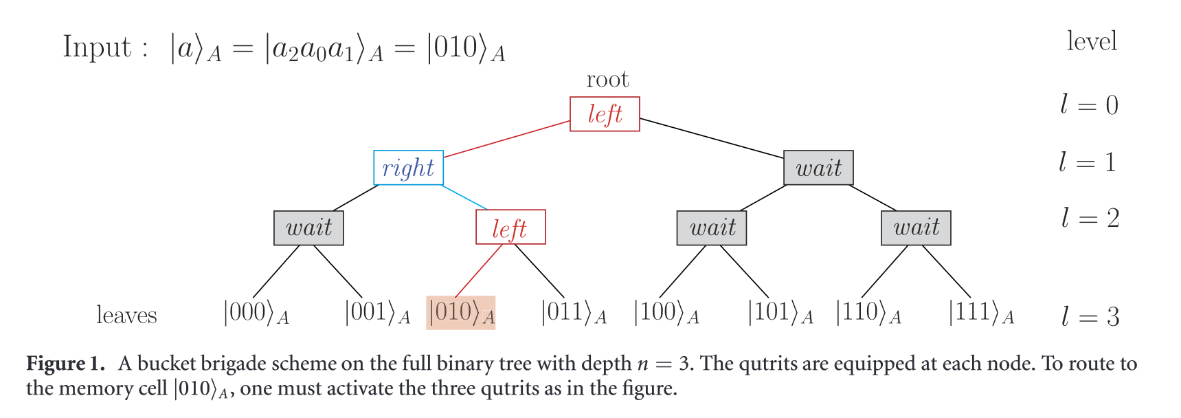
  • routing: a perfect binary tree with \(O(2^n)\) nodes

  • memory cells: \(2^n\) leaves

  • binary representation of the address: \(\ket{a_{n-1},\cdots,a_0}\), \(a_l=0\) left child, \(a_l=1\) right child

  • qutrit (left, right, wait) at each node

• scheme:

  1. routing \(O(n^2)\): \(a_l\) sequentially delivered from the root to a node at \(l\) th level and activates the qutrit to left / right; only \(n\) qutrits are activated

  2. querying: a quantum signal follows the path to the desired memory cell and retrieves information

  3. output: go back and reset the activated qutrits to state “wait”, obtains the output

QW on a binary tree:

• state:

  • bucket \(\ket{w,l}_B\): the \(w\) th node in level \(l\)

  • chirality \(\ket{c}_C\)

• space \(V_B\otimes V_C\):

  • bus space: \(V_B=\bigoplus_{w,l}V_{(w,l)}\ (V_{(w,l)}=\mathbb C)\) spanned by \(\ket{w,l}_B\)

  • chirality space: \(V_C=\mathbb C^2\)

  • address space: \(V_A=(\mathbb C^2)^{\otimes n}\)

• operator \(\mathcal S_{(w,l)}\in \mathscr L((V_{(w,l)}\oplus V_{(2w,l+1)}\oplus V_{(2w+1,l+1)})\otimes V_C)\):

  • forward:

    • \(\mathcal S_{(w,l)}\ket{w,l}_B\ket0_C=\ket{2w,l+1}_B\ket0_C\)

    • \(\mathcal S_{(w,l)}\ket{w,l}_B\ket1_C=\ket{2w+1,l+1}_B\ket1_C\)

  • backward:

    • \(\mathcal S_{(w,l)}\ket{2w,l+1}_B\ket0_C=\ket{w,l}_B\ket0_C\)

    • \(\mathcal S_{(w,l)}\ket{2w+1,l+1}_B\ket1_C=\ket{w,l}_B\ket1_C\)

  • keep:

    • \(\mathcal S_{(w,l)}\ket{2w,l+1}_B\ket1_C=\ket{2w,l+1}_B\ket1_CS_{(w,l)}\ket{2w,l+1}_B\ket1_C=\ket{2w,l+1}_B\ket1_C\)

    • \(\mathcal S_{(w,l)}\ket{2w+1,l+1}_B\ket0_C=\ket{2w+1,l+1}_B\ket0_C\)

  \[\begin{array}{l}\mathcal S_{(w,l)}=\sum\limits_{i=0}^1\left(\ket{2w+i,l+1}\bra{w,l}+\ket{w,l}\bra{2w+i,l+1}\right)_B\otimes\ket i\bra i_C\\+\sum\limits_{i=0}^1\ket{2w+\dfrac{1+(-1)^i}{2},l+1}\bra{2w+\dfrac{1+(-1)^i}{2},l+1}\otimes\ket i\bra i_C\end{array}\]

Contribution: employs a discrete-time quantum walk as a bucket brigade scheme

Algorithm

Representation:

• data stored in cell \(\ket{x^{(a)}}_D\):

  \(\ket{x^{(a)}}_D=\ket{x_{m-1}^{(a)}\cdots x_0^{(a)}}_D=\ket{x_{m-1}^{(a)}}_{D_{m-1}}\cdots\ket{x_0^{(a)}}_{D_0}\)

  \(\ket{x_i^{(a)}}\in V_{D_i}=\mathbb C^2\)

• address \(\ket a_A\):

  \(\ket{a}_A=\ket{a_{n-1}\cdots a_0}_A=\ket{a_{n-1}}_{A_{n-1}}\cdots\ket{a_0}_{A_0}\)

  \(\ket{a_i}\in V_{A_i}=\mathbb C^2\)

• space \(V:=V_B\otimes V_C\otimes V_A\otimes V_D\)

  • address space \(V_A\)

  • data space \(V_D\)

• qRAM: \(\sum\limits_{a\in \mathscr A}\ket{0,0}_B\ket 0_C\ket a_A\ket 0_D\mapsto \sum\limits_{a\in \mathscr A}\ket{0,0}_B\ket 0_C\ket a_A\ket{x^{(a)}}_D\)

  where \(\mathscr A\subset\{0,1,\cdots,2^n-1\}\)

• state:

  • initial state:

    \(\ket{\Psi_0^{(0)}}=\sum\limits_{a\in \mathscr A}\ket{0,0}_B\ket 0_C\ket a_A\ket 0_D\)

  • state at level \(l\): \(\ket{\Psi_0^{(l)}}\)

  • state with data: \(\ket{\Psi_x^{(n)}}\)

Schemes: qRAM = \(\mathcal{F^\dagger QF}\in\mathscr L(V)\)

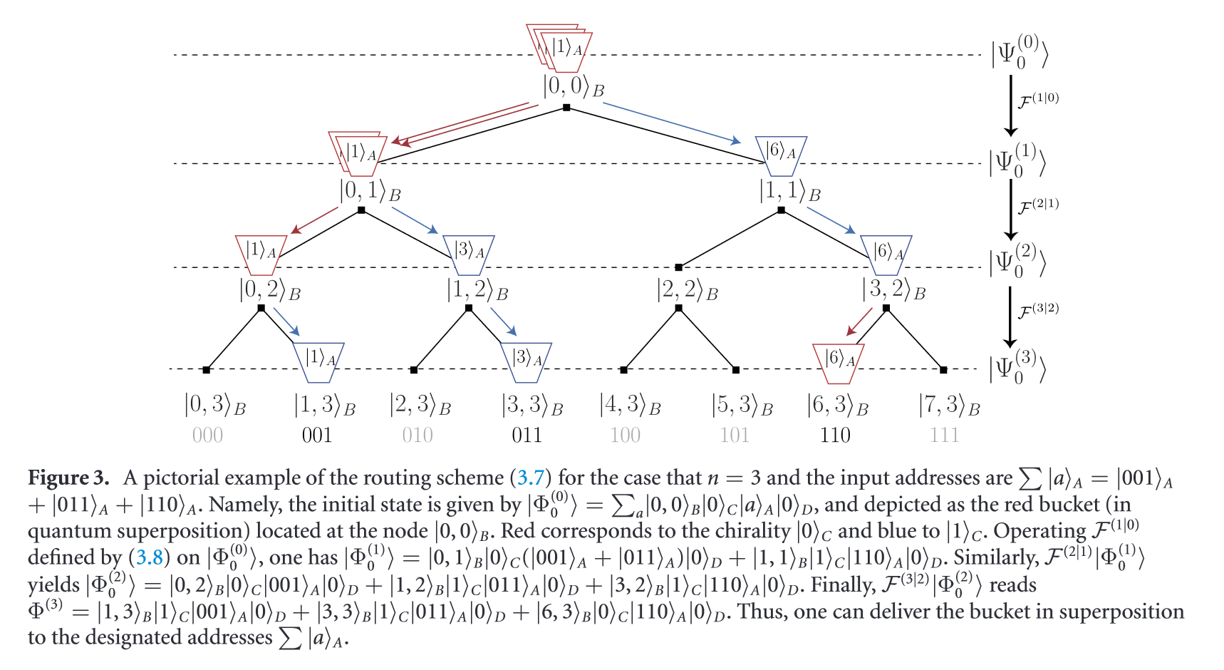
1. routing \(O(n)\): \(\ket{\Psi_0^{(n)}}=\mathcal F\ket{\Psi_0^{(0)}}\)

   • decomposed: \(\mathcal F=\mathcal F^{(n|n-1)}\cdots\mathcal F^{(1|0)}\)

     where \(\ket{\Psi_0^{(l+1)}}=\mathcal F^{(l+1|l)}\ket{\Psi_0^{(l)}}\)

   • plug \(a\) into \(w\), we have \(\ket{\Psi_0^{(l)}}:=\left|\sum\limits_{k=1}^l2^{l-k}a_{n-k},l\right\rangle_B\ket{a_{n-l}}_C\ket a_A\ket0_D\)

     \(a_{n-1}\) operates on the first layer with \(2^{l-1}\) effect on level \(l\)

   • \(\mathcal F^{(l+1|l)}:=\sum\limits_{w=0}^{2^l-1}\mathcal S_{(w,l)}\mathcal C_{C,A_{n-(l+1)}}\mathcal C_{C,A_{n-l}}\)

     NOT operator \(\mathcal C_{C,A_l}\in\mathscr L(V_C\otimes V_{A_l})\):

     \(\mathcal C_{C,A_l}:=I_C\otimes \ket0\bra0_{A_l}+X_C\otimes\ket1\bra1_{A_l},\ \mathcal C_{C,A_n}:=I_C\)

     \(\mathcal C_{C,A_{n-l}}\) clears \(a_{n-l}\) on chirality (\(c=0\)), \(\mathcal C_{C,A_{n-(l+1)}}\) loads \(a_{n-(l-1)}\) to chirality, then operates \(\mathcal S_{(s,w)}\) to shift

     thus

     \[\begin{array}{l}\ket{\Psi_0^{(0)}}=\sum\limits_{a\in \mathscr A}\ket{0,0}_B\ket 0_C\ket a_A\ket 0_D\xrightarrow{\mathcal F^{(1|0)}}\ket{\Psi_0^{(1)}}\cdots\\\xrightarrow{\mathcal F^{(n|n-1)}}\ket{\Psi_0^{(n)}}=\sum\limits_{a\in \mathscr A}\ket{a,n}_B\ket 0_C\ket a_A\ket 0_D\end{array}\]

     The motion of the shift operator is correspond with the address: \(a=\sum\limits_{k=1}^n2^{n-k}a_{n-k}\)

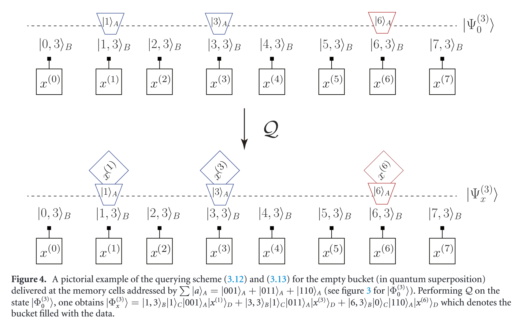
2. querying \(O(1)\): \(\ket{\Psi_x^{(n)}}=\mathcal Q\ket{\Psi_0^{(n)}},\mathcal Q\in\mathscr L(V_B\otimes V_D)\)

   \(\ket{\Psi_x^{(n)}}:=\sum\limits_{a\in \mathscr A}\ket{a,n}_B\ket 0_C\ket a_A\ket{x^{(a)}}_D\)

   • composed with Pauli X operator \(X_{D_i}\in\mathscr L(V_{D_i})\):

     \(\mathcal Q:=\sum\limits_{a=0}^{2^n-1}\ket{a,n}\bra{a,n}_B\otimes\left[\bigotimes\limits_{i=0}^{m-1}(X_{D_i})^{x_i^{(a)}}\right]\)

     \(\ket\cdot_B\) keeps the same, use \((X_{D_i})^{x_i^{(a)}}\) to change \(\ket\cdot_D\)

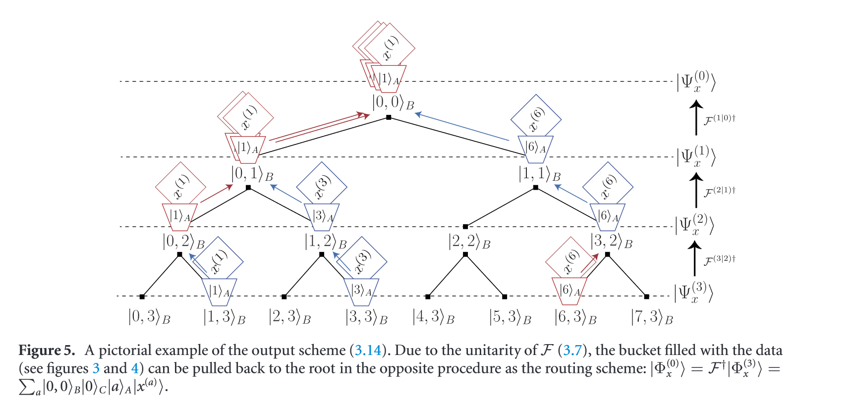
3. output: \(\mathcal F\) is unitary, \(\ket{\Psi_x^{(0)}}=\mathcal F^\dagger\ket{\Psi_x^{(n)}}\)

   where \(\ket{\Psi_x^{(0)}}=\sum\limits_{a\in \mathscr A}\ket{0,0}_B\ket 0_C\ket a_A\ket{x^{(a)}}_D\)

Example:

Implementation

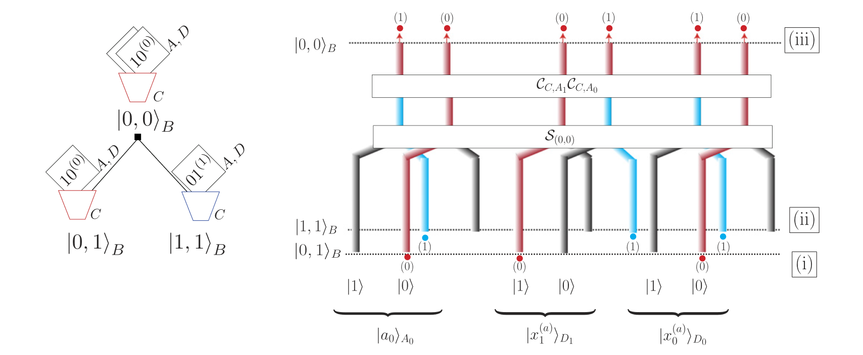
Dual-rail encoding: use \(2(n+m)\) rails to represent \(\ket c_C\ket a_A\ket{x^{(a)}}_D\)

• idea: using 2 rails (\(\ket1,\ket0\)) and 2 color to represent the qubits in \(\ket\cdot_A,\ket\cdot_D\)

  

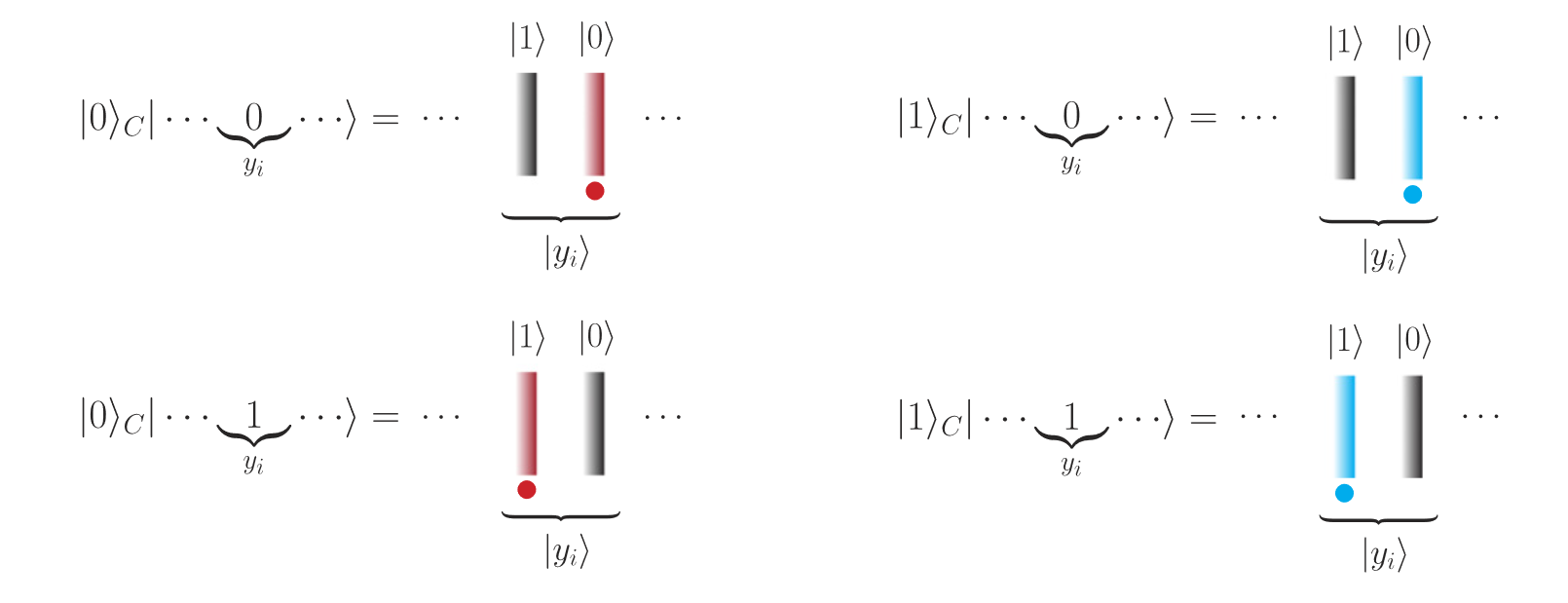
  where \(\ket\cdot_C\) controls the color of the rail, 0 for red, 1 for blue

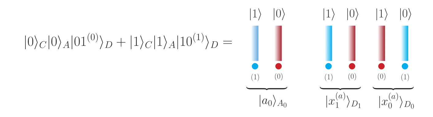
• superposition:

  

• example:

  \[\begin{array}{l}\mathcal F^\dagger:\ket{0,1}_B\ket0_C\ket0_A\ket{10^{(0)}}_D+\ket{1,1}_B\ket1_C\ket1_A\ket{01^{(1)}}_D\\\mapsto\ket{0,0}_B\ket0_C(\ket0_A\ket{10^{(0)}}_D+\ket1_A\ket{01^{(1)}}_D)\end{array}\]